A.Mary Selvam
Indian Institute of Tropical Meteorology, Pune, India
(Retired) email: selvam@ip.eth.net
website: http://www.geocities.com/amselvam
Applied Mathematical Modelling , 1993, Vol.17, 642-649
Abstract
A cell dynamical system model for deterministic chaos enables precise quantification of the round-off error growth,i.e., deterministic chaos in digital computer realizations of mathematical models of continuum dynamical systems. The model predicts the following: (a) The phase space trajectory (strange attractor) when resolved as a function of the computer accuracy has intrinsic logarithmic spiral curvature with the quasiperiodic Penrose tiling pattern for the internal structure. (b) The universal constant for deterministic chaos is identified as the steady-state fractional round-off error k for each computational step and is equal to 1 / t 2 ( =0.382) where t is the golden mean. k being less than half accounts for the fractal(broken) Euclidean geometry of the strange attactor. (c) The Feigenbaum's universal constants a and d are functions of k and, further, the expression 2a2 = p d quantifies the steady-state ordered emergence of the fractal geometry of the strange attractor. (d) The power spectra of chaotic dynamical systems follow the universal and unique inverse power law form of the statistical normal distribution. The model prediction of (d) is verified for the Lorenz attractor and for the computable chaotic orbits of Bernoulli shifts, pseudorandom number generators, and cat maps.
Keywords: deterministic chaos, strange
attractor, Penrose tiling pattern, cell dynamical system, universal algorithm
for chaos
1. Introduction
Nonlinear mathematical models of dynamical systems are sensitively dependent on initial conditions, identified as deterministic chaos. Such deterministic chaos was first identified nearly a century ago by Poincare1 in his study of the three-body problem. The advent of digital computers in the 1950s facilitated numerical solutions of model dynamical systems, and in 1963 Lorenz2 identified sensitive dependence on initial conditions in a simple mathematical model of atmospheric flows. Deterministic chaos occurs in both continuum(differential equations) and discrete (maps) systems. Deterministic chaos is now an area of intensive research in all branches of science and other areas of human interest3 . Ruelle and Takens4 identified deterministic chaos as similar to turbulence in fluid flows; turbulence is as yet an unresolved problem. It is well-known that deterministic chaos is a direct result of the following inherent limitations of numerical solutions: (a) The differential equations of traditional Newtonian continuum dynamics are solved as difference equations introducing space-time discretizations with implicit assumption of subgrid scale homogeneity for the dynamical processes. (b) Approximations in the governing equations related to limitations of computer capacity. (c) Exact number representation is not possible at the data input stage itself because of the binary form for number representation in computer arithmetic5 . (d) Computer-accuracy-related round-off errors magnify exponentially with time the above-mentioned uncertainties and give solutions that are not totally realistic6 . The trajectory of the dynamical system in the phase space traces a strange attractor, so named because its strange convoluted shape is the final destination of all possible trajectories. Trajectories starting from two initially close points diverge exponentially with time though still within the strange attractor domain. The strange attractor has self-similar geometry. The word fractal first coined by Mandelbrot7 means broken or fractured structure. The fractal dimension D of such non-Euclidean structure is given by the relation D = d ln M/d ln R where M is the mass contained within a distance R from a point within the fractal object. A constant value for D indicates uniform distribution of mass with distance on a logarithmic scale for the length scale R. Objects in nature in general possess a multifractal dimension8 . Self-similarity implies identical internal structure at all scales of magnification. The temporal fluctuations of dynamical systems have been investigated extensively and are found to exhibit a broad-band power spectrum9 . The physics of deterministic chaos is not as yet identified. In this paper, a cell dynamical system model for the growth of strange attractor pattern of deterministic chaos in dynamical systems is described by analogy with the formation of large eddy structures as envelopes enclosing turbulent eddies in fluid flows10,11 .
2. Computer accuracy and round-off error
Round-off error is inherent to finite precision numerical computations and imposes a limit dR to the resolution with which two quantities R + dR can be distinguished as separate, thereby introducing an uncertainty in computation equal to dR in magnitude. Computer precision dR is therefore analogous to yardstick length used in the measurement of distance of separation between two points. Two points cannot be distinguished as separate if they are closer together than the yardstick length dR used for the measurement. The uncertainty in measurement of separation distance of two points is equal to the yardstick length dR. Such round-off error is a direct consequence and the inevitable result of the necessity for discretization of space and time in traditional numerical computations and real-world measurements. In computer simulations of model dynamical systems, the negligibly small model input uncertainties are magnified by the round-off error and propagate into the mainstream computation with successive iterations because of the computational feedback logic inherent in such models, e.g., Xn+1 = F(Xn) where the value Xn+1 of the variable at the (n + 1)th interval is a function F of Xn . The uncertainty or its analogue, the yardstick length, dR, increases exponentially with each stage of computation and results in deterministic chaos as explained earlier. In the following discussions, computer precision is treated in terms of the equivalent yardstick length for length measurement. The computational domain is defined as equal to the product WR of the number of units of computation W of yardstick length R.
3. Cell dynamical system model for deterministic chaos
The round-off error structure growth, namely,
the strange attractor pattern in computed model dynamical systems , is
visualized as corresponding to the coherent structures such as large eddies
(or helical vortex roll circulations) that form as the envelopes of enclosed
turbulent eddies in planetary atmospheric boundary layer flows. Though
turbulent eddy fluctuations are considered to be chaotic(random) and dissipative,
they are an integral part of all organized coherent weather patterns such
as cloud rows/streets and the hurricane spiral cloud pattern. Townsend12
has shown that large eddy circulations form as a chance configuration of
turbulent eddy fluctuations in turbulent shear flows. Just as the small-scale
fluctuations contribute to the organized growth of large-eddy fluctuation
domains, so also the microscale round-off error structure domains contribute
to form the total uncertainty domain in the phase space of the model dynamical
system.
Computational error
is initiated with input data at the first step of numerical computation,
i.e., one unit of computation generates one unit of uncertainty equal to
the yardstick length dR in all directions as illustrated in Figure
1 by the circle OR2R1'R2 of
radius dR.
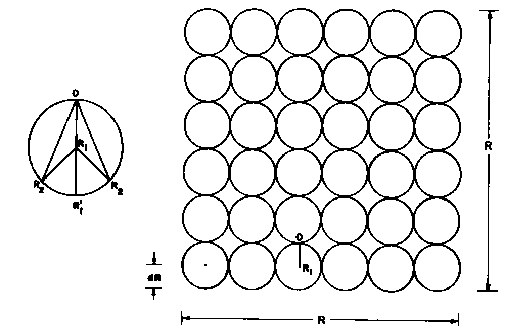
Figure 1. The growth
of round-off error structures in the phase space. The domain of the round-off
error dR is represented by the circle OR2R1'R2
on the left. The macroscale uncertainty domain of length scale R
is the sum of successive stages of such microscale round-off error domains
resulting from finite computer precision and shown by the close packing
of circles of radii dR on the right.
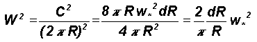
The uncertainty domain represented by the circle OR2R1'R2 corresponding to the measurement OR1 is interpreted as follows. One unit of measurement of yardstick length OR1 ( = dR ) implies two approximations: (a) a minimum measurable distance OR1 and (b) round-off of all lengths less than OR1' ( = 2dR ) as equal to OR1 ( = dR ). The domain of these two errors in the phase space is represented by a circle with center R1 and radius OR1 = dR because the projection of OR2 on OR1 for angles OR1R2 less than or greater than 90 degrees respectively will be measured as equal to OR1 . The circle OR2R1'R2 therefore represents the total uncertainty domain for one unit of measurement of yardstick length OR1 = dR . The precision decreases or the yardstick length R increases for with successive stages of computation. The increased imprecision represented by increased yardstick length R is composed of the microscale round-off error domain OR2R1'R2 as shown in Figure 1. Such microscopic error domain structures may be compared to turbulent eddy circulations, which contribute to form large eddy circulation patterns in fluid flows. w* units of computation of yardstick length dR is equivalent to W units of computation of a more imprecise larger yardstick length R and is quantified by analogy with the formation of large eddy circulation structures as the spatial average of the turbulent eddy fluctuation domain10-12 . The mean square round-off error circulation C2 at any instant around a circular path of length scale R is equal to the spatial integration of the microscopic domain error structures ( OR2R1'R2 ) over the computational domain of length scale R and is given as
![]()
The mean square value of W is then obtained as
or
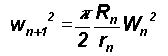
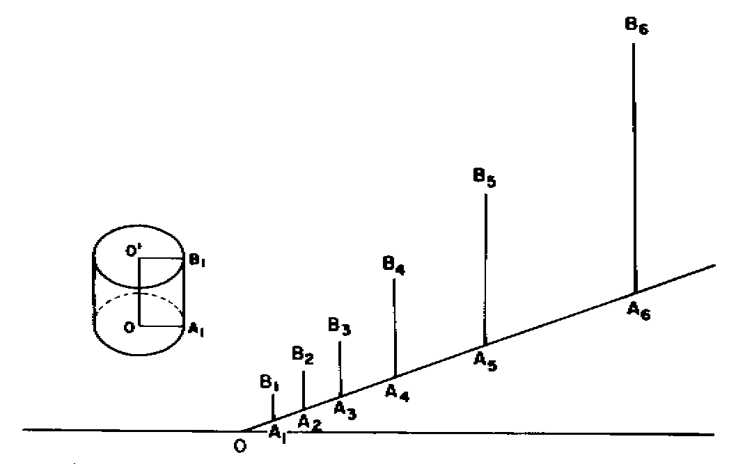
Figure 2. Visualization of round-off error growth in successive iterations
The uncertainty r1 in
the computation is equal to the number of units of computation W1,
i.e., r1 = 1 and is represented by A1A2
in Figure 2. The computation length OA1 can be
any radius of the sphere or circle in three or two dimensions respectively,
with center O and radius OA1 . The computational
domain W1R1 is any rectangular cross-section
OA1B1O'
of the cylinder with radius of base equal to OA1 and
height A1B1 (Figure 2). At the end
of the first step of computation W1 = 1, R1
= 1 and r1 = 1. Therefore W2 = 1.254
from equation (3). The first step of computation generates the length domain
R2
= R1 + r1 = 2 (OA2
= R2) associated with W2 = 1.254 units
of computation (A2B2 = W2)
and corresponding uncertainty, r2 = W2
= 1.254 (A2A3 = r2). Substitution
in equation (3) gives W3 = 1.985. Similarly the values
of Wn and Rn for the n
successive iteration steps are computed from equation (3). The yardstick
length Rn is equal to the cumulative sum of the yardstick
lengths for the previous
n intervals of computation, i.e., 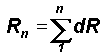 .
The values of Rn, Wn, dR, Wn+1,
and d q
computed as equal to Rn
/
Rn+1 and
.
The values of Rn, Wn, dR, Wn+1,
and d q
computed as equal to Rn
/
Rn+1 and 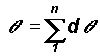 are tabulated in Table 1.
Table 1. The computed
spatial growth of the strange attractor design traced by dynamical systems
as shown in Figure 1.
|
|
|
|
|
|
|
|
2 3.254 5.239 8.425 13.546 21.780 35.019 56.305 90.530 |
1.254 1.985 3.186 5.121 8.234 13.239 21.286 34.225 55.029 |
1.254 1.985 3.186 5.121 8.234 13.239 21.286 34.225 55.029 |
0.627 0.610 0.608 0.608 0.608 0.608 0.608 0.608 0.608 |
1.985 3.186 5.121 8.234 13.239 21.286 34.225 55.029 88.479 |
1.627 2.237 2.845 3.453 4.061 4.669 5.277 5.885 6.493 |
It is seen that the yardstick length R and the corresponding number of units of computation W follow the Fibonacci mathematical number series. The progressive increase in imprecision represented by the increasing magnitude for the yardstick length can be plotted in polar coordinates as shown in Figure 3 where OR0 is the initial yardstick length.
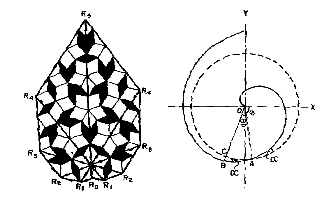
Figure 3. The quasiperiodic Penrose tiling pattern of the round-off error structure growth in the strange attractor. The phase space trajectory is represented by the product WR of the number of units of computation W of yardstick length R. R represents the round-off error in the computation. The successive values of W and R follow the Fibonacci mathematical number series, and the strange attractor pattern represented in this manner consists of the quasiperiodic Penrose tiling pattern. The overall envelope R0R1R2R3R4R5 of the strange attractor follows the logarithmic spiral R = re b q shown on the right where r = OR0 and b = tan a where a is the crossing angle.
The successively larger values of the yardstick
lengths are then plotted as the radii OR1, OR2
,OR3
,OR4
,and
OR5 on either side of OR0 such that the
angle between successive radii are
p
/ 5 so that the ratio of the successive yardstick lengths equals the golden
mean t
. The radii can be further subdivided into the golden mean ratio so that
the internal structure of the polar diagram displays the quasiperiodic
Penrose tiling pattern14. The larger yardstick length is therefore
shown to consist of microscale round-off error domains OR0R1
where
OR0
= R0R1 = dR.
dR is the imprecision
inherent to the computational system consisting of the model uncertainties
and the round-off error of the digital computer.
The computed result
WR
is represented by a rectangle of sides W and R, and therefore
the phase space trajectory can also be resolved into the quasiperiodic
Penrose tiling pattern. The spatial domain of the yardstick length OR0
is the solid of revolution generated by the rotation of the triangle OR1R0
about the axis
OR0 . It is seen from Table 1 and
Figure
3 that starting from either side of the initial computational step
OR0
the computation W proceeds in logarithmic spiral curves R0R1R2R3R4R5
such that one complete cycle is executed by the numerical computation after
five length steps of computation on either side of OR0
, i.e., clockwise and counterclockwise rotation. Denoting the yardstick
length scale ratio R/dR by Z, dominant periodicities or cycles
occur in the W units of computation for Z values in
multiples of t5n
where n ranges from positive to negative integer values. The internal
structure of the phase space trajectory , i.e., the strange attractor,
therefore consists of the quasiperiodic Penrose tiling pattern. The overall
envelope of the computation W follows the logarithmic spiral pattern.
The incremental units of computation dW of yardstick length R
at any stage of computation is non-Euclidean because of internal structure
generated by succesive stages of round-off error growth as shown in the
triangle OR0R1 (Figure 3). The incremental
units of computation dW of yardstick length R at any stage
of computation have intrinsic internal structure consisting of discrete
spatial domains of total size w*dR generated by w*
units of discrete yardstick length dR , which represents the uncertainty
in initial conditions, i.e., the error generated by assuming that the minimum
separation distance between two arbitrarily close points is equal to dR
.
At each stage of computation, the computed spatial domain RdW contains
smaller domains of total size w*dR representing the uncertainty
in input conditions, i.e., the error domains relating to the finite size
for yardstick length. The steady-state fractional round-off error k
in the computed model at each stage of computation is therefore given by
k also represents the steady-state
measure
of the departure from Euclidean shape of the computed model, namely, the
strange attractor. The successive computational steps generate angular
turning dq
of the W units of computation
where dq
= dR/R, which is a constant equal
to t
, the golden mean (Figure 3 ). Further, the successive values of
the W units of computation of yardstick length R follow Fibonacci
mathematical number series. k represents the steady-state fractional
error due to uncertainty in initial conditions coupled with finite precision
in the computed model. k also gives quantitatively the fractional
departure from Euclidean geometrical shape of the computed strange attractor
. k is derived from equation (4) as
k = 1/t2 = 0.382
A steady-state fractional round-off
error of 0.382 and the associated quasiperiodic Penrose tiling pattern
for the strange attractor are intrinsic to digital computations of nonlinear
mathematical models of dynamical systems even in the absence of uncertainty
in input conditions for the model. Because the steady-state fractional
departure from Euclidean shape of the strange attractor design traced in
the phase space by W units of computation is equal to 0.382, i.e.,
less than half, the overall Euclidean geometrical shape of the strange
attractor is retained. Beck and Roepstroff15 also find the universal
constant 0.382 for the scaling relation between length of periodic orbits
and computer precision in numerical computations. k , which is a
function of the golden mean t
, is hereby identified as the universal constant for deterministic chaos
in computer realizations of mathematical models of dynamical systems. k
is independent of the magnitude of the precision of the digital computer
and, also, the spatial and temporal length steps used in model computations.
In Section 4 it is shown that the Feigenbaum's universal constants16
are functions of k . Dominant coherent structures in numerical computation
W
evolve for yardstick length scale ratio Z equal to t5n
(n ranging from negative to positive integer values) as mentioned
earlier and are characterized by round-off error-generated quasiperiodic
Penrose tiling pattern for the internal structure. Numerical experiments
have identified the golden mean t
to be associated with deterministic chaos in dynamical systems17,18.
Also, recent numerical investigations indicate that the strange attractor
can be defined completely as quasiperiodicities with fine structure19,
i.e., a continuum.
Traditional computational
techniques are digital in concept, i.e., they require a unit or yardstick
for the computation and thereby lead inevitably to approximations, i.e.,
round-off errors. Because the computed quantity structure can be infinitesimally
small in the limit, there exists no practical lower limit for the yardstick
length. Therefore, numerical computations in the long run give results
that scale with computer precision and also give quasiperiodic structures.
Numerical experiments show,that, due to round-off errors, digital computer
simulations of orbits of chaotic atractors will always eventually become
periodic5. The expected period in the case of fractal chaotic
attractors scales with round-off20. The universal quantification
of the round-off error structure growth described in this paper is independent
of the magnitude of the roud-off error, the time and space increments,
and the details of the nonlinear differential equations and, therefore,
is universally applicable for all computed model dynamical systems.
The incremental growth
dW
units of numerical computation of yardstick length R can be expressed
in terms of w* units of more precise yardstick length
dR
as follows from equation(4):
Equation (6) can be integrated to obtain
the
W units of total computation starting with w*
units of yardstick length r ,where, as mentioned earlier,
dR
represents the uncertainty in initial conditions of the computational system
at the beginning of the computation.
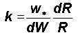
The W units of computation
and therefore R follow a logarithmic spiral with Z being
the yardstick length scale ratio, i.e., Z = R/dR . The logarithmic
spiral R0R1R2R3R4R5
(Figure 3) is given quantitatively in terms of the yardstick length
R
as
![]()
where b = tan a
with a
,
the crossing angle equal to dR/R
. a
is therefore equal to 1/t
as shown earlier and, because b is equal to a
in the limit for small increments
dW
in computation,
![]()
The yardstick length R, which
represents uncertainty in initial conditions, therefore grows exponentially
with progress in computation. The separation distance r of two arbitrarily
close points at the beginning of the computation grows to R at the
end of the computation with the angular turning of the trajectories being
equal to p
/ 5 . The exponential divergence
of two arbitrarily close points is given quantitatively by the exponent
1/t
equal to 0.618 and is identified as the Lyapunov exponent conventionally
used to measure such divergence in computed dynamical systems17.
For each length of computation with unit angular turning (equal to
p
/ 5 ) the initial yardstick
length r increases to 1.855r (from equation (9)) at the end
of the computation, i.e., the yardstick length (or round-off error) approximately
doubles for each iteration when the phase space trajectory is expressed
as the product WR where W units of computation of yardstick
length R follow the Fibonacci mathematical number series as a natural
consequence of the cumulative addition of round-off error domains. Hammel
et
al.21 mention that it is not unusual that the distance between
two close points roughly doubles on every iterate of numerical computation.
The Lyapunov exponent equal to 1/t
(= 0.618) is intrinsic to numerically computed systems even in the
absence of uncertainty in initial conditions for the numerical model. When
uncertainty in input conditions exists for the model dynamical system,
the initial yardstick length r effectively becomes larger and, therefore,
larger divergence of initially close trjectories occurs for a shorter length
step of computation as seen from equation (9). The generation of strange
attractor in computer realizations of nonlinear mathematical models is
a direct consequence of computer-precision-related round-off errors. The
geometrical structure of the strange attractor is quantified by the recursion
relation of equation (2). Equation (2) is hereby identified as the universal
algorithm for the generation of the strange attractor pattern with underlying
universality quantified by the Feigenbaum's universal constants16a
and d in computer realizations of nonlinear mathematical models
of dynamical systems. In the following section it is shown quantitatively
that equation (2) gives directly the universal characteristics such as
the Feigenbaum's constants identifying deterministic chaos of diverse nonlinear
mathematical models.
4. Universal algorithm for deterministic chaos incorporating Feigenbaum's universal constants
The basic example with the potential to display the main features of the erratic behavior characterizing deterministic chaos is the Julia model given below
Xn+1 = F(Xn) = LXn(1 - Xn)
The above nonlinear model represents
the population values of the parameter X at different time periods
n
, and L parameterizes the rate of growth of X for small X
. Feigenbaum's research16 showed that the two universal
constants a and d are independent of the details of the nonlinear
equation for the period doubling sequences
![]()
![]()
In the above equation ![]() denotes the X spacing between adjoining period doublings
(n+2) and (n+1), i.e.,
denotes the X spacing between adjoining period doublings
(n+2) and (n+1), i.e., ![]() and similarly
and similarly ![]() .
. ![]() is the L
spacing between period doublings (n+2) and (n+1) . The universal
recursion relation quantifying deterministic chaos in nonlinear mathematical
models, namely, equation (2) is analogous to the Julia model, because the
macroscale computation structure W is determined by the microscopic
yardstick length dR . The Feigenbaum's constants a
and d for the universal period doubling route to chaos may
be derived directly from the universal recursion relation (equation (2))
as shown in the following. The universal relation (equation (2))
is used for computing quantitatively the successive length step increments
in the magnitude of the number of units of computation w*
of yardstick length dR incorporated in the computation.
is the L
spacing between period doublings (n+2) and (n+1) . The universal
recursion relation quantifying deterministic chaos in nonlinear mathematical
models, namely, equation (2) is analogous to the Julia model, because the
macroscale computation structure W is determined by the microscopic
yardstick length dR . The Feigenbaum's constants a
and d for the universal period doubling route to chaos may
be derived directly from the universal recursion relation (equation (2))
as shown in the following. The universal relation (equation (2))
is used for computing quantitatively the successive length step increments
in the magnitude of the number of units of computation w*
of yardstick length dR incorporated in the computation.
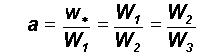
Feigenbaum's constant
a
is given by the successive spacing ratios W for adjoining
period doublings. W and R are respective successive
spacing ratios , because by definition W and R
are computed as incremental growth steps dW and dR
for each stage of computation.
Feigenbaum's constant
a
is obtained as the successive spacing ratios of W , i.e.,
The total computational domain WR
at any stage of computation may be considered to result from spatial integration
of round-off error domain W1R1 or W2R2
where R1 and R2 refer
to the precision. From equation (2) W12R1
= W22R2 = constant. Therefore

From equations (4) and (5)
a = 1/k = t 2
The Feigenbaum's constant a
therefore denotes the relative increase in the computed domain with respect
to the yardstick length (round-off error) domain and is equal to
t
2 (=2.618)
and is inherently negative because the round-off error has a negative sign
by convention.
Further,
2a 2
= total variance of the fractional geometrical evolution of computed domain
for both clockwise and counterclockwise phase space trajectories.
The Feigenbaum's constant
d
is the successive spacing ratios of R for the universal recursion
relation(equation (2)) for the numerical computation.
Because W12R1 = W22R2 as explained above
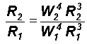
The Feigenbaum's constant d is therefore obtained as
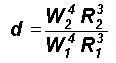
W 4
represents the fourth moment about the reference level for the instantaneous
trajectory in the representative volume R 3 of
the phase space. d is, therefore, equal to the relative volume
intermittency of occurrence of Euclidean structure in the phase space during
each computational step, i.e., p /
5 radian angular rotation as
shown earlier in Table 1 for the quasiperiodic Penrose tiling pattern
traced by the strange attractor. For one complete cycle(period) of computation,
five length steps of simultaneous clockwise and counterclockwise, i.e.,
counter-rotating, computations are performed. Therefore, for one complete
cycle of computation the relative volume intermittency of occurrence of
Euclidean structure in the computed phase space domain is
p
d
. The universal recursion relation for deterministic chaos(2) can be written
as
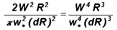
The reformulated universal algorithm
for numerical computation at equation (15) can now be written in terms
of the universal Feigenbaum's constants (equations (13) and (14)) as
2a2 = p d
The above equation states that the
relative volume intermittency of occurrence of Euclidean structure for
one dominant cycle of computation contributes to the total variance of
the fractional Euclidean structure of the strange atractor in the phase
space of the computed domain. Numerical computations by Delbourgo22
give the relation
2a2 = 3d, which is almost identical
to the model-predicted equation (16).
Feigenbaum's universal
constants a = 2.503 and d = 4.6692 (equations
(11) and (12)) have been determined by numerical computations at period
doublings n, n+1 and n+2 where n is large.
At large n, computational difficulties in resolution of adjacent
period doublings impose a limit to the accuracy with which a
and d can be estimated.
The Feigenbaum's constants
a
and d computed from the universal algorithm
2a2
= p d
refer to an infinitesimally small value for the computer round-off-error(yardstick
length), i.e., an infinitely large number of period doublings. The model-predicted
and computed a and d are therefore not identical.
5. Universal quantification for the power spectra of chaotic dynamical systems
The temporal fluctuations of chatic dynamical systems are found to exhibit broad-band power spectra9. A complete description of the temporal variability is therefore possible in terms of the component periodicities and their phases19. Such a description in terms of cycles or periodicities of nonlinear fluctuations of real world dynamical systems has been reported23. In the following, it is shown that the power spectra of the nonlinear fluctuations of chaotic dynamical systems can be quantified in terms of the universal characteristics of the statistical normal distribution. Because the successive number of units of computation W is obtained as the R.M.S. value of inherent round-off error domains as given in equation (1), the mean square variance W 2 for the continuum of computed W will follow normal distribution characteristics. The model predictions are in agreement with continuous periodogram analysis24 of the Lorenz attractor25 and the computable chaotic orbits of (a) Bernoulli shifts, (b)cat maps, and (c) pseudorandom number generators5 . The details of the mathematical equations of the computable chaotic dynamical systems5 used is given in the following:
1. Bernoulli shifts
2. Cat mapx ----> 3x mod 1,(x0, x1,......, xn,...)with x0 = 0.1
3. Pseudorandom number generator: minimal standard Lehmer generatorF(x, y) = (x + y mod 1, x + 2y mod 1)with initial points(0.1,0.0)for all 0<= x, y < 1
Xn+1 = 16807 Xn mod 2147483647; X0 = 0.1
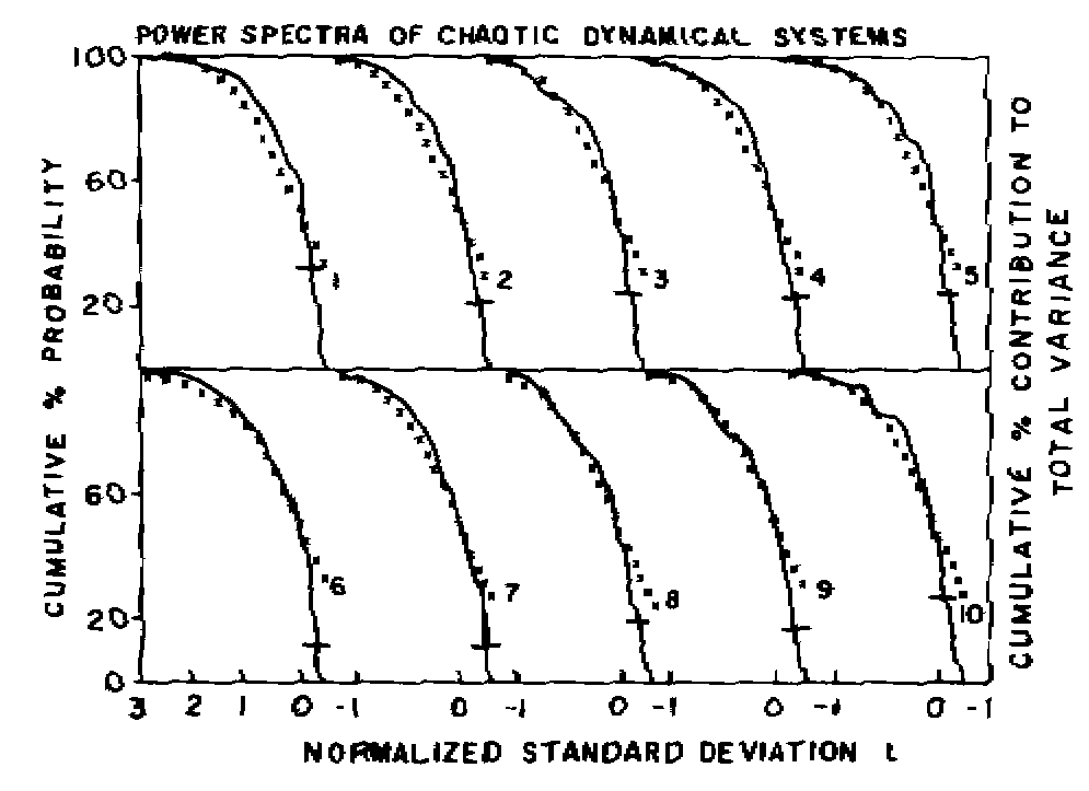
The power spectra of the above chaotic dynamical systems(Figure 4) are found to be the same as the normal probability density distribution with the normalized variance representing the eddy probability density corresponding to the normalized standard deviation t equal to [(log P/log P50) - 1] where P is the period and P50 , the period up to which the cumulative percentage contribution to total variance is equal to 50. The above relation for the normalized standard deviation t in terms of the periodicities follows directly from equation (7) because by definition W and W 2 represent respectively the standard deviation and variance as a direct consequence of W being computed as the instantaneous average round-off error domains for each stage of computation. Therefore, for a constant value of w* , the number of units of computation of precision dR , the ratio of the R.M.S. units of computation W1 and W2 of respective yardstick lengths R1 and R2 will give the ratios of the standard deviations of the unit W of computation. From equation (7)
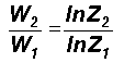
Starting with reference level standard
deviation
s
equal to W1,
the successive steps of computation have standard deviations W2
equal to s
, 2s
, 3s
, .....from equation (17) where
Z2
= Z1n and n = 1, 2, 3, ....for successive
period doubling growth sequences.
The important result
of the present study is the quantification of the round-off error structure,
namely, the strange attractor in model dynamical systems in terms of the
universal and unique characteristics of the statistical normal distribution.
The power spectra of the Lorenz attractor and the computable chaotic orbits
of the Bernouille shifts, pseudorandom number generators, and cat map exhibit
(Figure 4) the universal inverse power law form of the statistical
normal distribution. The inverse power law form for the power spectra of
the temporal fluctuations is ubiquitous to real-world dynamical systems
and is recently identified as the temporal signature of self-organized
criticality26 and indicates long-range temporal correlations
or non-local connections. Sensitive dependence on initial conditions, i.e.,
deterministic chaos, is therefore a manifestation of self-organized criticality
in model dynamical systems and is a natural consequence of the spatial
integration of microscopic domain round-off error structures as postulated
by the cell dynamical system model described in Section 3. The universal
quantification for deterministic chaos, or self-organized criticality in
terms of the unique inverse power law form of the statistical normal distribution
identifies the universality underlying numerical computations of chaotic
dynamical systems. The total pattern of fluctuations of chaotic dynamical
systems is predictable, because self-organization of the nonlinear fluctuations
of all scales contributes to form the unique pattern of the normal distribution
(Figure 4).
6. Conclusion
In summary, the cell dynamical system model for round-off error growth in computer realizations of nonlinear dynamical systems visualizes the computer precision (round-off error) as analogous to yardstick length in length measurement. The computed domain consists of the cumulative integrated mean of enclosed round-off error domains. The computed domain, namely, the phase space trajecory, is the product WR of the number of units of computation W of precision (yardstick length) R . The phase space trajectory thus defined traces an overall logarithmic spiral pattern with the golden mean winding number and quasiperiodic Penrose tiling pattern for the internal structure, implying long-range temporal correlations, namely, sensitive dependence on initial conditions. The universality underlying deterministic chaos is quantified in terms of the following universal constants, which are functions of the golden mean t : (1) The constant k for deterministic chaos equal to 1 / t 2 represents the steady-state fractional round-off error for each computational step. k also represents the fractional departure from Euclidean geometry of the strange attractor. (2) The Lyapunov exponent is equal to 1 / t . (3) The Feigenbaum's constants a and d define the algorithm for deterministic chaos as 2a 2 = p d , which states that the relative volume intermittency of occurrence equal to p d of fractional Euclidean structure contributes to the total variance equal to 2a 2 of the strange attractor. a is equal to t 2 and represents the fractional Euclidean structure of the strange attractor. (4) The power spectra of computed chaotic dynamical systems follow the universal inverse power law form of the statistical normal distribution. Continuous periodogram power spectral analysis of Lorenz attractor, Bernouille shifts, pseudorandom number generators, and cat maps are in agreement with model predictions.
Acknowledgements
The author is grateful to Dr.A.S.R.Murty for his keen interest and encouragement during the course of this study. Thanks are due to Shri R.Vijayakumar for assistance with computer graphics and to Shri M.I.R.Tinmaker for typing the manuscript.
References
1 Poincare, H. Les
meyhodes nouvelle de la mecanique celeste. Gautheir-Villars,
Paris, 1892
2 Lorenz, E. N. J.
Atmos.Sci.
(1963), 20, 130
3 Gleick, J. Chaos:
Making a New Science. Viking, New York, 1987
4 Ruelle, D. and Takens,
F. Commun. Math. Phys. 1971, 20, 167
5 Palmore, J. and
Herring, C. Physica D 1990, 42, 99
6 Stewart, I. Nature
1992, 355, 16
7 Mandelbrot, B. B.
PAGEOPH 1989, 131 (1/2), 5
8 Stanley, H. E. and
Meakin, P. Nature 1988, 335, 405
9 Procaccia, I. Nature
1988, 333, 618
10 Selvam, A. Mary,
Can. J. Phys.
1990, 68, 831
11 Selvam, A. Mary, Pethkar, J.
S. and Kulkarni, M. K. Int. J. Climatol. 1992, 12, 137
12 Townsend, A. A. The Structure
of Turbulent Shear Flow. Cambridge University Press, Cambridge, 1956
13 Oona, Y. and Puri, S. Phys.
Rev. A. 1988, 38, 434
14 Janssen, T. Phys.
Rep. 1988, 168, 1
15 Beck, C. and Roepstorff,
G. Physica D 1987, 25, 173
16 Feigenbaum, M. J.
Los
Alamos Sci. 1980, 1, 4
17 McCauley, J. L. Physica
Scripta 1988, T20, 1
18 Stewart, I. New
Scientist 1992, 135, 14
19 Cvitanovic, P. Phys.
Rev. Lett. 1988, 61, 2729
20 Grebogi, C., Ott,
E. and Yorke, J. A. Phys. Rev. A 1988, 38, 3688
21 Hammel, S. M., Yorke,
J. A. and Grebogi, C. Amer. Math. Soc. 1988, 19(2), 465
22 Delbourgo, R. Asia-Pacific
Physics News 1986, 1, 7
23 Olsen, L. F. and
Schaffer, W. M. Science 1990, 249, 499
24 Jenkinson, A. F.
A powerful elementary method of spectral analysis for use with monthly,
seasonal or annual meteorological time series. U. K. Meteorol. Office,
Met. O 13 Branch Memorandum No. 57, 1977, p.23
25 Blackadar, A. Weatherwise
1990 43(4),210
26 Bak, P., Tang, C.
and Wiesenfeld, K. Phys. Rev.A 1988, 38, 364