Universal Spectrum for Natural Variability of Climate : Implications for Climate Change

J. S. Pethkar and A. M. Selvam^*

Indian Institute of Tropical Meteorology, Pune 411008, India  

Amer. Meteorol. Soc.10th Conf. Applied Climatology, Fall 1997, Western USA.

^*(Retired) email: selvam@ip.eth.net

web site: http:\\www.geocities.com\amselvam 

1.      INTRODUCTION  

      The apparently irregular ( unpredictable ) space-time fluctuations in atmospheric flows ranging from climate ( thousands of kilometers - years ) to turbulence ( millimeters - seconds ) exhibit the  universal symmetry of selfsimilarity. Selfsimilarity or scale invariance implies long-range spatiotemporal correlations and is manifested in atmospheric flows as the fractal geometry to spatial pattern concomitant with inverse power-law form for power spectra of temporal fluctuations documented and discussed in detail by Lovejoy and his group (Tessier et. al. 1996). Long-range spatiotemporal correlations are ubiquitous to dynamical systems in nature and are identified as signatures of self-organized criticality (Bak et. al.1988). Standard meteorological theory cannot explain satisfactorily the observed self-organized criticality. Numerical models for simulation and prediction of atmospheric flows are subject to deterministic chaos and give unrealistic solutions. Deterministic chaos is a direct consequence of round-off error growth in iterative computations. Round-off error of finite precision computations doubles on an average at each step of iterative computations ( Mary Selvam 1993a). Round-off error will propagate to the mainstream computation and give unrealistic solutions in numerical weather prediction (NWP) and climate models which incorporate thousands of iterative computations in long-term numerical integration schemes. A recently developed non-deterministic cell dynamical system model for atmospheric flows (Mary Selvam 1990) predicts the observed self-organized criticality as intrinsic to quantumlike mechanics governing flow dynamics.  

2.   MODEL CONCEPTS

                In summary, (Mary Selvam 1990,1993a,b ,1997; Mary Selvam et. al. 1992,1996; Mary Selvam, Pethkar and Kulkarni 1995; Mary Selvam and Radhamani 1994,1995; Mary Selvam and Joshi 1995), based on Townsend's ( Townsend 1956) concept that large eddies are the envelopes of enclosed turbulent eddy circulations, the relationship between the large and turbulent eddy circulation speeds (W and w_* ) and radii ( R and r ) respectively is given as                                                       

(1)

Since the large eddy is the integrated mean of enclosed turbulent eddy circulations, the eddy energy (kinetic) spectrum follows statistical normal distribution. Therefore, square of the eddy amplitude or the variance represents the probability. Such a result that the additive amplitudes of eddies, when squared, represent the probability densities is obtained for the subatomic dynamics of quantum systems such as the electron or photon (Maddox 1988a). Atmospheric flows, therefore, follow quantumlike mechanical laws. Incidentally, one of the strangest things about physics is that we seem to need two different  kinds of mechanics, quantum mechanics for microscopic dynamics of quantum systems and classical mechanics for macroscale phenomena (Rae 1988).The above visualization of the unified network of atmospheric flows as a quantum system is consistent with Grossing’s (Grossing 1989) concept of quantum systems as order out of chaos phenomena. Order and chaos have been reported in strong fields in quantum systems (Brown 1996). Writing Equation 1 in terms of the periodicities  T and  t of large and small eddies respectively,  where

            and

we obtain                                                              

(2)

Equation 2 is analogous to Kepler’s third law of planetary motion, namely, the square of the planet’s year (period) to the cube of the planet’s mean distance from the Sun is the same for all planets (Narlikar 1982,1996; Weinberg 1993). Newton developed the idea of an inverse square law for gravitation in order to explain Kepler’s laws, in particular, the third law. Kepler’s laws were formulated on the basis of observational data and therefore were of empirical nature. A basic physical theory for the inverse square law of gravitation applicable to all objects, from macroscale astronomical objects to microscopic scale quantum systems is still lacking. The model concepts (Eq.2) are analogous to a string theory (Kaku 1997) where, superposition of different modes of vibration result in material phenomena with intrinsic quantumlike mechanical laws which incorporate inverse square law for inertial forces, the equivalent of gravitational forces, on all scales of eddy fluctuations from macro- to microscopic scales.

Uzer et al.(1991) have discussed new developments within the last two decades which have spurred a remarkable revival of interest in the application of classical mechanical laws to quantum systems. The atom was originally visualized as a miniature solar system based on the assumption that the laws of classical mechanics apply equally to electrons and planets. However within a short interval of time the new quantum mechanics of Schrodinger and Heisenberg became established (from the late 1920s) and the analogy between the structure of the atom and that of the solar system seemed invalid and classical mechanics became the domain of the astronomers. There is now a revival of interest in classical and semiclassical methods which are found to be unrivaled in providing  an intuitive and computationally tractable approach to the study of atomic, molecular and nuclear dynamics.

2.1    Model Predictions

(a)     Atmospheric flows trace an overall logarithmic spiral trajectory with the quasiperiodic Penrose tiling pattern for the internal structure

(b)     Conventional continuous periodogram power spectral analyses of such spiral trajectories will reveal a continuum of periodicities with progressive increase in phase.

(c)     The broadband power spectrum will have embedded dominant wave-bands, the bandwidth increasing with period length. The peak periods E_n in the dominant wavebands will be given by the relation

E_n = T_s(2+t)tⁿ                                                                                           (3)

where t is the golden mean equal to (1+Ö5)/2 [@1.618] and T_s , the solar powered primary perturbation time period is the annual cycle (summer to winter) of solar heating in the present study of interannual variability. Ghil (1994) reports that the most striking feature in climate variability on all time scales is the presence of sharp peaks superimposed on a continuous background.

The model predicted periodicities are 2.2, 3.6, 5.8, 9.5, 15.3, 24.8, 40.1, and 64.9 years for values of n ranging from -1 to 6. Periodicities close to model predicted have been reported (Burroughs 1992; Kane 1996).

(d)     The ratio  r/R  also represents the increment  dq  in phase angle q (Equation 1 )and therefore the phase angle q  represents the variance. Hence, when the logarithmic spiral is resolved as an eddy continuum in conventional spectral analysis, the increment in wavelength is concomitant with increase in phase. Such a result that increments in wavelength and phase angle are related is observed in quantum systems and has been named 'Berry's phase' (Berry 1988; Maddox 1988b). The relationship of angular turning of the spiral to intensity of fluctuations is seen in the tight coiling of the hurricane spiral cloud systems.

(e)     The overall logarithmic spiral flow structure is given by the following relation containing the length scale ratio z equal to R/r

(4)

where the constant k is the steady state fractional volume dilution of large eddy by inherent turbulent eddy fluctuations . The constant  k  is equal to 1/t² (@ 0.382) and is identified as the universal constant for deterministic chaos in fluid flows. The steady state emergence of fractal structures is therefore equal to

1/k @ 2.62                                                                 (5)

          The model predicted logarithmic wind profile relationship such as Equation 4 is a long-established (observational) feature of atmospheric flows in the boundary layer, the constant k, called the Von Karman ’s constant has the value equal to 0.38 as determined from observations. Historically, Equation 4 is basically an empirical law known as the universal logarithmic law of the wall , first proposed in the early 1930s by pioneering aerodynamicists Theodor von Karman and Ludwig Prandtl, describes shear forces exerted by turbulent flows at boundaries such as wings or fan blades or the interior wall of a pipe. The law of the wall has been used for decades by engineers in the design of aircraft, pipelines and other structures (Cipra, 1996).

          In Equation 4, W represents the standard deviation of eddy fluctuations, since W  is computed as the instantaneous r.m.s. (root mean square) eddy perturbation amplitude with reference to the earlier step of eddy growth. For two successive stages of eddy growth starting from primary perturbation w_*  the ratio of the standard deviations W_n+1  and W_n is given from Equation 4 as (n+1)/n. Denoting by s  the standard deviation of eddy fluctuations at the reference level (n=1) the standard deviations of eddy fluctuations for successive stages of eddy growth are given as integer multiple of s,  i.e.,  s, 2s, 3s, etc. and correspond respectively to

statistical normalized standard deviation   t   = 0, 1, 2, 3, etc.        (6)

The conventional power spectrum plotted as the variance versus the frequency in log-log scale will now represent the eddy probability density on logarithmic scale versus the standard deviation of the eddy fluctuations on linear scale, since the logarithm of the eddy wavelength represents the standard deviation i.e., the r.m.s. value of eddy fluctuations (Equation 4). The r.m.s. value of eddy fluctuations can be represented in terms of statistical normal distribution as follows. A normalized standard deviation t=0 corresponds to cumulative percentage probability density equal to 50 for the mean value of the distribution. Since the logarithm of the wavelength represents the r.m.s. value of eddy fluctuations the normalized standard deviation  t  is defined for the eddy energy as

(7)

where  L  is the period in years and  T₅₀  is the period up to which the cumulative percentage contribution to total variance is equal to 50 and  t = 0. The variable logT₅₀  also represents the mean value for the r.m.s. eddy fluctuations and is consistent with the concept of the mean level represented by r.m.s. eddy fluctuations. Spectra of time series of meteorological parameters when plotted as cumulative percentage contribution to total variance versus t should follow the model predicted universal spectrum. The literature shows many examples of pressure, wind and temperature whose shapes display a remarkable degree of universality (Canavero and Einaudi,1987).

(f)      Mary Selvam (1993a) has shown that Equation 1 represents the universal algorithm for deterministic chaos in dynamical systems and is expressed in terms of the universal Feigenbaum's (Feigenbaum 1980) constants  a  and  d  as follows.

2a² = p d                                                                  (8)

where p d , the relative volume intermittency of occurrence contributes to the total variance 2a² of fractal structures. The Feigenbaum’s constant a represents the steady state emergence of fractal structures. Therefore, the total variance of fractal structures for either clockwise or anticlockwise rotation is equal to 2a². It was shown at Equation 5 above that the steady state emergence of fractal structures in fluid flows is equal to   1/k( = t²) and therefore the Feigenbaum’s constant  a is equal to

a = t² = 1/k = 2.62                                                     (9)

(g)     The relationship between Feigenbaum’s constant a and statistical normal distribution for power spectra is derived in the following.

The steady state emergence of fractal structures is equal to the Feigenbaum’s constant a (Equation 5 ). The relative variance of fractal structure for each length step growth is then equal to a². The normalized variance  1/a²ⁿ   will now represent the statistical normal probability density for the n^th step growth according to model predicted quantumlike mechanics for fluid flows . Model predicted probability density values P are computed as

P = t ^{- 4n}                                                                       (10)

or

P = t ^{- 4t}                                                                      (11)

where t is the normalized standard deviation (Equation 6) and are in agreement with statistical normal distribution as shown in Table 1.  

Table 1

Model predicted and statistical normal probability density distributions

                The periodicities T₅₀ and T₉₅ up to which the cumulative percentage contribution to total variances are respectively equal to 50 and 95 are computed from model concepts as follows.

                The power spectrum, when plotted as  normalised standard deviation t versus cumulative percentage contribution to total variance represents the statistical normal distribution (Equation 7), i.e., the variance represents the probability density. The normalised standard deviation values corresponding to cumulative percentage probability densities P equal to 50 and 95 respectively are equal to 0 and 2 from statistical normal distribution characteristics. Since t represents the eddy growth step n (Equation 6) the dominant periodicities T₅₀ and T₉₅ up to which the cumulative percentage contribution to total variance are respectively equal to 50 and 95 are obtained from Equation 3 for corresponding values of n , i.e., 0 and 2. In the present study of interannual variability, the primary perturbation time period T_s is equal to the annual (summer to winter) cycle of solar heating and T₅₀ and T₉₅ are obtained as

T₅₀ = (2+t)t⁰ @ 3.6 years                                             (12)

T₉₅ = (2+t)t² @ 9.5 years                                             (13)

(h)     The power spectra of fluctuations in fluid flows can now be quantified in terms of universal  Feigenbaum’s  constant  a  as follows.

The normalized variance and therefore the statistical normal distribution is represented by (from Equation 11)

P = a ^{- 2t}                                                                      (14)

where  P  is the probability density corresponding to normalized standard deviation  t. The graph of P versus t will represent the power spectrum. The slope  S  of the power spectrum is equal to

(15)

The power spectrum therefore follows inverse power law form, the slope decreasing with increase in t. Increase in t corresponds to large eddies ( low frequencies) and is consistent with observed decrease in slope at low frequencies in dynamical systems.

(I)      The fractal dimension  D can be expressed as a function of the universal Feigenbaum’s  constant  a  as follows.

The steady state emergence of fractal structures is equal to a for each length step growth (Equations 6 & 9) and therefore the fractal structure domain is equal to a^m at m^th  growth step starting from unit perturbation. Starting from unit perturbation, the fractal object occupies spatial (two dimensional) domain a^m associated with radial extent t^m since successive radii follow Fibonacci number series. The fractal dimension D is defined as

where  M  is the mass contained within a distance  R  from a point in the fractal object. Considering growth from  n^th   to  (n+m)^th   step

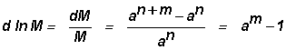
(16)

similarly

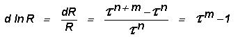
(17)

Therefore from Equation 9

(18)

The fractal dimension increases with the number of growth steps. The dominant wavebands increase in length with successive growth steps. The fractal dimension D indicates the number of periodicities incorporated. Larger fractal dimension indicates more number of periodicities and complex patterns.

(j)            The relationship between fine structure constant, i.e. the eddy energy ratio between successive dominant eddies and Feigenbaum’s constant a is derived as follows.

 2a² = relative variance of fractal structure (both clockwise and anticlockwise rotation) for each growth step.

For one dominant large eddy comprising of five growth steps each for clockwise and counterclockwise rotation,  the total variance is equal to

2a² x 10 = 137.07                                                    (19)

For each complete cycle ( comprising of five growth steps each ) in simultaneous clockwise and counterclockwise rotations, the relative energy increase is equal to 137.07 and represents the fine structure constant for eddy energy structure.

Incidentally ,the fine structure constant in atomic physics (Davies 1986; Gross 1985; Omnes 1994) designated as a ^{- 1} , a dimensionless number equal to 137.03604 is very close to that derived above for atmospheric eddy energy structure. This fundamental constant has attracted much attention and it is felt that quantum mechanics cannot be interpreted properly until such time as we can derive this physical constant from a more basic theory.

(k)     The ratio of proton mass M to electron mass m_e , i.e.,  M/m_e is another fundamental dimensionless number which also awaits derivation from a physically consistent theory. M/m_e determined by observation is equal to about 2000. In the following it is shown that ratio of energy content of large to small eddies for specific length scale ratios is equivalent to M/m_e.

From Equation 19,

The energy ratio for two successive dominant eddy growth = (2a² x10)²

Since each large eddy consists of five growth steps each for clockwise and anticlockwise rotation,

The relative energy content of primary circulation structure inside this large eddy

= (2a² x 10)²/10   @ 1879

The cell dynamical system model concepts therefore enable physically consistent derivation of fundamental constants  which define the basic structure of quantum systems. These two fundamental constants could not be derived so far from a basic theory in traditional quantum mechanics for subatomic dynamics (Omnes 1994).

3.      APPLICATIONS FOR PREDICTION

(a)           In a majority of spectra, periodicities up to 4 years contribute up to 50% of total variance (see references of Mary Selvam et. al.) and is in agreement with model prediction (Equation 12) The model also predicts that  periodicities up to 9.5 years contribute up to 95% of total variance( Equation 13). Dominant periodicities, such as the widely documented QBO, ENSO and decadal scale fluctuations may be used for predictability studies.

(b)           Model predicted universal spectrum (Equation 7) has been identified in the interannual variability of rainfall (Mary Selvam et al. 1992; Mary Selvam 1993b; Mary Selvam et al. 1995); temperature (Mary Selvam and Joshi 1995) and surface pressure (Mary Selvam et al. 1996) and imply laws analogous to Kepler’s laws (Equation 2) for eddy circulation dynamics. Universal spectrum for atmospheric interannual variability provides precise quantification for the apparently irregular natural variability. The concept of universal spectrum for fluctuations rules out linear secular trends in meteorological parameters with regard to climate change. Global warming, either natural or man - made (industrialization related) will result in enhancement of fluctuations of all scales (Equation 1).The following studies indicate intensification of space-time fluctuations in atmospheric flows in recent years (since 1970s). Intergovernmental Panel on Climate Change (IPCC)  report shows that recent increases have been found in the intensity of the winter atmospheric circulation over the extratropical Pacific and Atlantic (Houghton et al 1996).There have been relatively more frequent El Nino episodes since 1976/77 with only rare excursions into the other extreme (La Nina episodes) An assessment of ENSO - scale secular variability shows that ENSO - scale variance is relatively large in recent decades (Wang and Ropelewski 1995). Hurrel and Van Loon (1994) have reported a delayed breakdown of the polar vortex in the troposphere and lower stratosphere after the late 1970s coincident with the beginning of the ozone deficit in the Antarctic spring. It is possible that enhanced vertical mixing (Equations 6 and 7) inside the polar vortex may contribute to the ozone loss. Regions of enhanced convective activity in the monsoon regime are found to be associated with lower levels of atmospheric columnar total ozone content (Hingane and Patil 1996). Incidentally, it was found that enhancement of background noise, i.e., energy input into the eddy continuum results in amplification of faint signals in electrical circuits (Brown 1996).

4.       ACKNOWLEDGEMENTS

          The authors express their gratitude to Dr. A.S.R. Murty for his keen interest and encouragement during the course of this study

5.      REFERENCES

Bak, P. C., C. Tang, and K. Wiesenfeld, 1988: Self-organized criticality, Phys. Rev. A. 38, 364 - 374.

Berry, M. V.,1988: The geometric phase. Sci. Amer.  Dec., 26-32.

Brown, J.,1996: Where two worlds meet. New Scientist, 18 May, 26-30.

Burroughs, W. J.,1992: Weather Cycles: Real or Imaginary? Cambridge University Press, Cambridge.

Canavero, F. G., and  Einaudi, F.,1987: Time and space variability of atmospheric processes. J. Atmos. Sci., 44(12) ,1589-1604.

Cipra, B., 1996: A new theory of turbulence causes a stir among experts. Science, 272, 951.

Davies, P. C. W.,1986: The Forces of Nature. 2nd Edn. Cambridge University Press, Cambridge.

Feigenbaum , M. J.,1980: Universal behaviour in nonlinear systems. Los Alamos Sci.  1 , 4 - 27.

Ghil, M.,1994: Cryothermodynamics : the chaotic dynamics of paleoclimate. Physica D 77,130-159.

Gross, D. J.,1985: On the uniqueness of physical theories. In A Passion for Physics. (Eds.) De Tar, C., Finkelstein, J., and Tan, C-I. World Scientific, Singapore.

Grossing , G.,1989: Quantum systems as order out of chaos phenomena. Il Nuovo Cimento 103B , 497 - 510.

Hingane, L. S., and S. D. Patil, 1996: Total ozone in the most humid monsoon region. Meteorol. Atmos. Phys., 58, 215-221.

Houghton, J. T., L. G. Meira Filho, B. A. Callandar., N. Harris, A. Kattenberg, and Maskell, K., 1996: Climate Change 1995 , Intergovernmental Panel on Climate Change. Cambridge University Press, Cambridge.

Hurrel, J. W., and H. Van Loon, 1994: A modulation of the atmospheric annual cycle in the southern hemisphere. Tellus, 46A, 325-338.

Kaku, M., 1997: Into the eleventh dimension. New Scientist, 18 Jan. 32-36.

Kane, R. P., 1996: Quasibiennial and quasitriennial oscillations in some atmospheric parameters. PAGEOPH 147(3) , 567-583.

Maddox, J., 1988a: License to slang Copenhagen ? Nature, 332, 581.

Maddox, J., 1988b: Turning phases into frequencies, Nature, 334 ,99 .

Mary Selvam, A.,1990: Deterministic chaos, fractals and quantumlike mechanics in atmospheric flows. Can. J. Phys., 68, 831-841.  http://xxx.lanl.gov/html/physics/0010046

Mary Selvam, A., J. S. Pethkar, and M. K. Kulkarni, 1992: Signatures of a universal spectrum for atmospheric interannual variability in rainfall time series over the Indian region. Int'l . J. Climatol., 12, 137-152.

Mary Selvam, A.,1993a: Universal quantification for deterministic chaos in dynamical systems. Applied Math. Modelling, 17 , 642-649.  http://xxx.lanl.gov/html/physics/0008010

Mary Selvam, A.,1993b: A universal spectrum for interannual variability of monsoon rainfall over India. Adv. Atmos. Sci., 10 ,  221-226.

Mary Selvam, A., and M. Radhamani, 1994: Signature of a universal spectrum for nonlinear variability in daily columnar total ozone content. Adv. Atmos. Sci., 11(3) ,  335-342.

Mary Selvam , A., J. S. Pethkar, and M. K. Kulkarni, 1995: Some unique characteristics of atmospheric interannual variability in rainfall time series over India and the United Kingdom. Adv. Atmos. Sci., 12(3) , 377 - 385.

Mary Selvam, A., and M. Radhamani , 1995: Universal spectrum for short period (days) variability in atmospheric total ozone. Mausam , 46(3) , 297 - 302.

Mary Selvam, A., and R. R. Joshi,1995: Universal spectrum for interannual variability in COADS global air and sea surface temperatures. Int'l. J. Climatol., 15 , 613 -624.

Mary Selvam, A., J. S. Pethkar, M. K. Kulkarni, and R. Vijayakumar, 1996: Signatures of a universal spectrum for atmospheric interannual variability in COADS surface pressure time series. Int'l.  J. Climatol.,16 , 1 - 11.

Mary Selvam, A.,1998: Quasicrystalline pattern formation in fluid substrates and phyllotaxis, In Symmetry in Plants, Barabe, D., and R. V. Jean , (Eds.), World Scientific Series in Mathematical Biology and Medicine, Vol.4., World Scientific, Singapore, pp.795-809.  http://xxx.lanl.gov/abs/chao-dyn/9806001

Narlikar, J. V., 1982: Violent phenomena in the universe. Oxford University Press, Oxford, pp. 213.

Narlikar, J. V., 1996: The lighter side of gravity. Cambridge University Press, Cambridge, pp. 217.

Omnes, R., 1994:The Interpretation of Quantum Mechanics. Princeton University Press, Princeton NJ .

Rae, A., 1988: Quantum-physics: illusion or reality ? Cambridge University Press,New York,p.129.

Tessier, Y., S. Lovejoy, P. Hubert, D. Schertzer, and S. Pecknold, 1996: Multifractal analysis and modelling of rainfall and river flows and scaling, causal transfer functions. J. Geophys. Res., 101(D21), 26427-26440.

Townsend, A. A.1956. The Structure of Turbulent Shear Flow, Cambridge University Press,  London, U.K.

Uzer , T .,  Farrelly , D., Milligan , J. A., Raines, P. E., and Skelton, J. P.,1991: Celestial mechanics on a microscopic scale. Science, 253 , 42 - 48.

Wang, X. L., and Ropelewski, C. F., 1995: An assessment of ENSO-scale secular variability. J. Climate  8(6), 1584-1599.

Weinberg, S., 1993: Dreams of a final theory. Vintage, pp.250.